LOCAL ADAPTIVITY AND QUASI-OPTIMAL DISCRETIZATIONS
FOR MULTIVARIATE ISOGEOMETRIC ANALYSIS

WE PRESENT:
1.
Drawback of traditional methods
2.
Overview about Isogeometric Analysis
3.
Local refinements and non-conformity
4.
Quasi-optimal choice of the refinement type
5.
Results for single patches
6.
Spline Multigrid solver
|
1. Drawback of traditional methods:
|
Classical methods for simulation use as input a mesh which
is triangular or quadrilateral in 2D and which is tetrahedral or hexahedral in
3D. They have several disadvantages which are related to
geometry and
hierarchy:
-
Those traditional methods require dense meshes not only in order to
attain a good accuracy for solving the PDE but also to obtain a good
approximation of the physical geometry. Indeed, in order to obtain
an accurate representation of the used geometries, an initial mesh is
usually taken. For real world CAD objects, a large number of gridpoints
are required in order to have a good approximation of the geometries.
The resulting polygonal or polyhedral approximation, usually
denoted by Ω, is considered as the initial mesh of simulation.
Depending on the accuracy required for the PDE simulation, the domain
Ω still needs to be further refined by using some a-posteriori
error estimator. Hence,
an unnecessarily large degree of freedom.
-
To overcome the above problem, traditional methods take a very coarse
mesh which is a polyhedral or polygonal approximation. That mesh is then
repeatedly updated by shifting boundary nodes to the exact geometry.
That is, nodes are translated toward the boundary when boundary refinements
occur. Such a refinement technique can be easily applied to convex
domains such as spheres or cylinders. When the domain has a concave
boundary, shifting a boundary node to a curved boundary could cause an
interference such as mesh folding because the new boundary node might well
be inside some triangle. The resulting mesh interference has to be corrected.
Thus, one has to apply a difficult geometric rectification
on the fly beside solving the PDE.
-
Many numerical analysts are fond
of hierarchy on account of its efficiency. In the context of
hierarchical methods like multigrid, multilevel or multiscale, one needs
a sequence of hierarchical nested finite dimensional spaces such as

Traditional methods suffer from difficult problems in generating such a
hierarchical structure because the only available data are
usually the finest space. Algorithms for mesh
simplification (or geometry decimation) using multiresolution techniques do
exist. However, they enable only the sequence of meshes to become
coarser and coarser. The sequence of corresponding
finite dimensional spaces are in general not nested
Return to content
|
2. Overview about Isogeometric Analysis:
|
|
|
The most widely used representations in CAD are Bézier,
B-spline, Coons, Gordon, and NURBS patches. NURBS entities have become
a CAD standard because they can describe the other representations
exactly. In addition, with very few control points NURBS enables exact
representations of algebraic entities like circular arcs, spheres,
conic sections which are important components of CAD assemblies. Hence,
NURBS entities become the most supported components in modern CAD exchange
standards such as IGES or STEP. The IGA is featured by three good properties:
-
CAD integration:
it enables the coupling of simulation and modeling on the same
CAD model.
-
Small geometric degree of freedom:
it does not increase the degree of freedom to capture geometric
accuracy. It keeps the CAD domain of simulation unchanged from
starting until finishing the computation.
-
Hierarchical solver:
it enables hierarchical solvers like multigrid even for complicated
CAD objects. The sequence of nested spaces can be easily generated
while projection and restriction operators are fast to compute.
|
|
Return to content
|
3. Local refinements and non-conformity:
|
The input is a small number of NURBS surfaces or solids
Mi
defined on parameter domains P
i which can be supposed to be the unit
square or the unit cube. The treatment of the PDE carries the problem from the
physical domain over to the parameter domain P. The entries of the Jacobian
matrix of each NURBS mapping and the one for its inverse can be exactly
computed even if the value of the inverse of the NURBS is unknown. The problem
is completely solved on the parameter domain. For the spaces of approximation,
the original IGA (see for e.g. works of Hughes, Basilevs, Buffa) uses NURBS
functions as bases. But here we restrict ourselves to B-splines which are
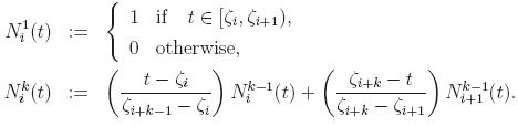
For the multivariate case where the dimension is
d=2 or
d=3, we
use the following bases

Hence, the space of approximation within a single B-spline domain is given by

Let us note that the main weakness of IGA so far is that it uses
global refinements instead of
local ones. Global refinements
imply that an insertion of a knot entry in one direction spreads along the
whole range of the other directions. Not only such a process increases the
degree of freedom but the shape regularity condition of the spline segments
could be violated. To circumvent such a problem, we allow our discretization to
be
non-conforming. In addition, the approximation space on one parameter
domain
P is given by

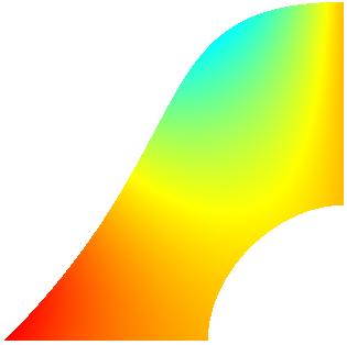
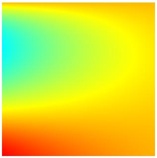
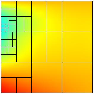
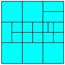
A typical simulation on a single 2D patch is illustrated in the next
figure. On the left figure, the physical NURBS patch is displayed with
the exact solution. The middle figure shows the exact solution on the
parameter domain. On the right figure we see some non-conforming
discretization obtained from a certain sequence of local refinements
together with the corresponding computed solution.
The main properties of our implementation are summarized as follows:
-
Full adaptivity using a-posteriori error estimator,
-
Use of local refinements,
-
Optimal element distribution,
-
Hierarchical solver.
Return to content
|
4. Quasi-optimal choice of the refinemen type:
|
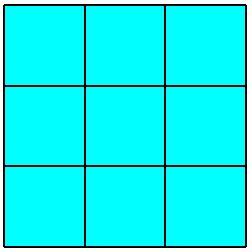
We construct an automatic self-adaptive discretization which
starts from an initial mesh that is always supposed to be a very coarse tensor
product mesh. We use an a-posteriori error estimator which permits to evaluate
the numerical errors without knowing the exact solution. Only elements
admitting too large errors need to be refined. That avoids the need of global
uniform refinements. In order to evaluate the error within an element
Q
of the mesh on each patch, we use the following estimator for a
d-dimensional
problem where
d=2,3.
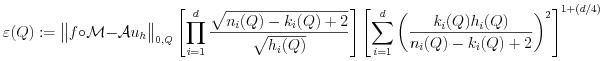
where
f is the RHS,
M describe the NURBS patch
parametrization,
A is obtained from the Laplace operator, (
ni
(
Q),
ki(
Q)) are the spline properties on the
x
i-direction of the element
Q and
hi(
Q)
is the length of the element
Q on the
xi-direction.
Afterwards, the elements
Q having the largest value of the above estimator
are refined in order to obtain a new mesh. When an element in the mesh needs to
be refined, it is not known beforehand which kind of refinement ought to be applied.
There are several possibilities for refinements. One can apply subdivisions on different directions. One can also insert new knot entries. The choice of the type of refinement
should dynamically depend on both the solution of the PDE to be solved and the NURBS
blocks. We introduced a method for choosing an optimal refinement which would
reduce the error most in the next mesh. Optimality is not understood in the
strict sense that there is no other discretization which yields a more accurate
result. Optimality here is gauged with respect to some constant frames which
depend only on the current discretization. Suppose that the current solution in
u
h. Consider a larger space
E where the solution is u
E.
It is evident that u
E is at least as accurate as u
h. We
search for the space
E which has the largest error reduction. It is
clear that a very small deviation of u
E from u
h could
produce only a very small error reduction as in
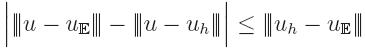
Therefore, we should try to maximize that deviation so that the error is
likely to be reduced most. Unfortunately, u
E is unknown
and it makes no sense to compute it on a finer mesh for every possible mesh.
Therefore, we need to find a way to gauge the deviation. Based on hierarchical
spline space decompositions, we use the following estimates
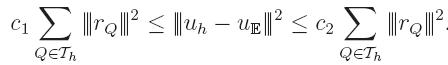
Here, the constants c
1 and c
2 do not depend on the
refinement type or position. In addition, the determination of the
estimator r
Q amounts to solving a system which is linear, which
is symmetric positive definite and which is very small.
Return to content
|
5. Results for single patches:
|
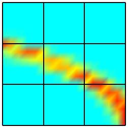
We present now a few refinement results on single patches.
First, we consider the following exact solutions which correspond respectively
to an internal layer and to an internal accumulation. The RHS of the Laplace
equation are computed accordingly. Inside some tight positions of the domains,
those functions admit unity values. Elsewhere, they decay exponentially to
zero. The size of the internal features can be controlled by the parameter ω.
The NURBS function which describes the patch is exactly the same as the one in
Section 3. The position of the layer can be controlled by the parameter
c.
Similarly, the one for the internal accumulation by the parameters
(a,b).

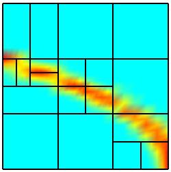
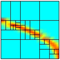
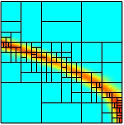
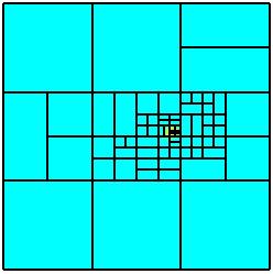
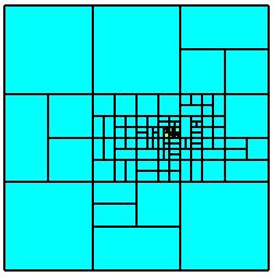
Repeated applications of the refinement process yield the
following sequence of discretizations on the parameter domain. Further results
including numerical comparison with global refinements and with uniform
discretizatrions as well as 3D simulations can be found in our papers.
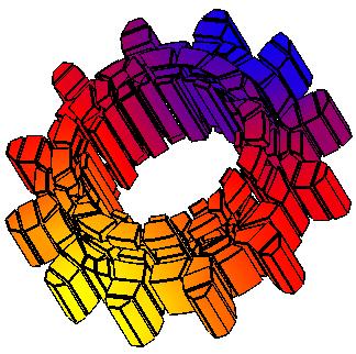
The second refinement sequence plainly illustrates the geometric
situation in Section 1 where there is no need to perform a refinement
next to the boundary although the geometry has curvilinear boundaries.
Return to content
|
6. Spline multigrid linear solver:
|
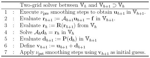
The corresponding linear system is solved by using a modified multigrid
algorithm. Below, we summarize the two-grid case which uses two nested
spaces. The difference from the standard two-grid method is about the
restriction and prolongation operators
R and
P. For the
standard two-grid, some templates combining neighboring nodal values are
used. Such a nodal combination cannot be used here because there are
no nodes inside the elements. The multigrid process consists in applying
the two-grid operation several times during the coarse grid correction.
-
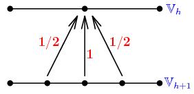
Use discrete B-splines for the prolongation operator P,
-
Use non-uniform spline-wavelets for the restriction operator R,
-
Use the same pre-smoothing and post-smoothing method as in standard multigrid,
-
Use the same coarse grid correction as in standard multigrid.
Here, we use the Gauss-Seidel iteration for those smoothing
steps. We numerically investigated that spline multigrid whose convergence
history until the 21-st iteration is displayed in the next Table. We examine
also the corresponding error at each iteration as well as the ratio between the
errors of two consecutive iterations.
| ITERATION | ERROR | RATIO BTW. CONSEC. ERRORS |
| 0 | 2.558340e+000 | nothing |
| 3 | 2.932692e-005 | 10.433512 |
| 6 | 4.572813e-008 | 5.410555 |
| 9 | 7.159492e-010 | 3.048095 |
| 12 | 2.787349e-011 | 2.837645 |
| 15 | 1.242582e-012 | 2.800942 |
| 18 | 5.710444e-014 | 2.717146 |
| 20 | 7.999520e-015 | 2.386161 |
| 21 | 3.352464e-015 | 1.940152 |
Return to content
Last Update: on March 31st, 2010, in Bonn, by Maharavo Randrianarivony.