NONLINEAR POISSON-BOLTZMANN: modeling, adaptivity, multilevel.
|
OVERVIEW ABOUT IONIC PROBLEM:
|
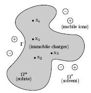
We consider the interaction of solute and solvent media which are
respectively denoted by Ωu and Ωv. The
surface Γ represents the solute-solvent boundary which is in our case the
Connolly surface. The solute is located inside the cavity composed of immobile
charges while the external domain is constituted of mobile ions. Our ongoing and
future objectives:
- Modeling of data acquired from PDB (Protein Data Bank),
- Coarse curved tetrahedral patches from the Connolly surface,
- Nonlinear correction with fast convergence,
- FFT and FHT(Fast Hartley Transform) based nonlinear solver,
- A-posteriori error estimator and adaptive refinement,
- Higher order elements using Dubiner bases.
|
|
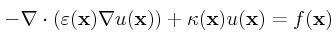
We consider the following nonlinear PDE admitting the unknown u, related
to the electrostatic potential, on the ionic solution
Ω=ΩuUΩ
v:
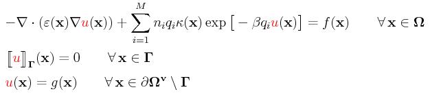
The coefficients ε(x) and κ(x) are
space-dependent functions related to the dielectric
value and the modified Debye-Hueckle parameter. Those coefficients might be
highly discontinuous between Ωu and Ωv
but the jump of solution u is required to be zero across the interface
Γ. The value of ni is the
number density of counter-ions of type i and qi is its charge
while β:=1/(kBT) with kB and T being the
Boltzmann constant and the temperature.
|
|
For real chemical simulation, the right-hand expression f(x)
is related to the internal electric charges while the boundary function
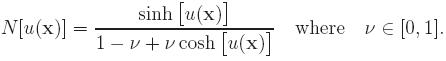
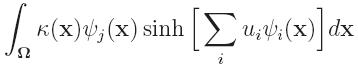
g is zero. But for our numerical models, we let them general for comparison reason. In the monovalent case, the above nonlinear expression
is replaced by sinh. If the solvent ions are assumed
to occupy sites on a lattice, the nonlinear expression is
|
|
In the monovalent case, by considering only the first term of the Taylor expansion,
one obtains the
linear (or linearized)
Poisson-Boltzmann equation:
Such an approximation of
sinh yields
very inaccurate results for highly charged
electrostatic potentials. As a consequence, we consider the
nonlinear Poisson-Boltzmann equation (PBE).
|
MODELING AND DATA ACQUISITION FROM PDB:
|
For our simulation, we use two kinds of geometric discretization:
- Unstructured meshes composed of fine tetrahedra. In this
case, the simulation is performed at the physical domains.
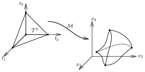
- Hierarchical representation: we decompose the domains into
curved parametric tetrahedral patches and we simulate at
the parametric domains.
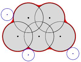
Both methods require some geometric preparation. The geometric information
are acquired from the Van der Waals radii and the PDB files containing the
coordinates of the nuclei. We need a weighted Voronoi
decomposition. For two spheres B1(m1,r1) and B2(m2,r2), we use the
power distance

|
|
|
With respect to the power distance, one can tessellate the whole
space into weighted Voronoi cells (Laguerre). This decomposition
is obtained by using the convex hull in
R4 of the initial points added with weights.
The weighted Delaunay is used to derive the
decomposition where you use the orthocenter
and the orthoradius of the projection of the weighted
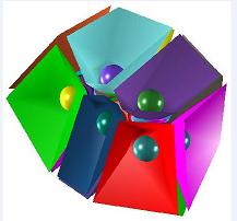
convex hull. After the initial decomposition process, the molecular surfaces
are represented as composite trimmed surfaces. Each one of them is composed
of one base NURBS surface and a few NURBS curves which trim the base NURBS surface.
Thus, the raw trimmed surfaces typically have several sides and internal holes.
For the unstructured meshes, we need to apply usual techniques for the
generation of the tetrahedra. As for the hierarchical case, more care must
be considered.
|
|
In most interesting cases where the probe radius is about 1.4 Angstrom and the number of atoms
are more than 50, there are typically many trimmed surfaces (toroidal and spherical) which
are very thin. As a consequence, the usual approach about decomposing the trimmed surfaces
into fine triangles which are then tetrahedralized does not function anymore. More accurately, that is still valid but it produces tetrahedra which are undesirable for subsequent numerical
simulation. What we need are block tetrahedra which are large enough and well shaped.
For some related works, follow the next links:
For the unstructured case, we treat a single mesh for the whole simulation
domain. The simulation is thus performed directly on the
Ω.
As for the multiblock version, our treatment has the next properties:
We have a nested sequence of finite sequence of finite dimensional spaces:

- We do not use a single mesh for the whole model but rather many parametric meshes
(one for each curved tetrahedra),
- The results in a coarser structure is used to enhance those in a fine one,
- In the course of the refinement, we keep track of the the parent/children
hierarchy: which tetrahedra of Vk correspond to elements of
Vk+1,
- We organize our data structure and code structure efficiently so as to treat
the hierarchical refinements patch by patch.
|
SEQUENCE OF NONLINEAR PROBLEMS:
|
A related work is the method of Xie et al:
Xie and Zhou: A new minimization protocol for solving nonlinear
Poisson-Boltzmann mortar finite element equation,
(BIT Numerical Mathematics (2007) 47: 853�871)
This is a very good source for the mortar case but it has serious
drawbacks. For Xie et al, in order to solve the nonlinear optimization,
they evaluate on the fly the integrals
by using some numerical quadrature where ψj is some
FE-bases. As a consequence, the evaluations of the
objective functional, gradient and the Hessian are either very
expensive or inaccurate. That method is still feasible in the
2D case if the model is very small as they considered. To remedy
those drawbacks, our PBE nonlinear solver is featured by
- Quasi-Newton based on BFGS,
- Efficient and accurate line search,
- Fast-Fourier Transform Hessian,
- Nonlinear correction with fast convergence.
|
|
We use a method avoiding numerical quadrature on the fly for functional, gradient
or Hessian evaluations. We replace the initial problem by a sequence of nonlinear
problems which are simpler to solve. If we assume that we have an approximation
uh(k), the next approximation is obtained
by solving for the correction function
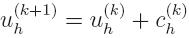
|
leading to
|
|
For the solving of the simplified nonlinear problem for c(k)h,
we use an improved quasi-Newton method which is not computationally expensive since
there are no integrals
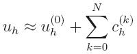
to be estimated. At first sight, the above sum looks expensive
but it turns out that only very few terms of that sum are necessary to
obtain a good accuracy.
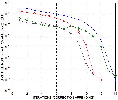
Nonlinear solver for unstructured mesh:
On the right plots, you see some instances of
the convergence for the case of unstructured meshes. We consider
various values of the parameters seen in the type of Poisson-Boltzmann
equation.
|
|
The convergence has the following typical feature: it is
dragging down slowly until it reaches a certain closeness and then it drops
very quickly. In case of hierarchy the convergence is much faster
because the starting slow convergence is removed. Below are some
results for the hierarchical case.
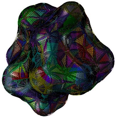
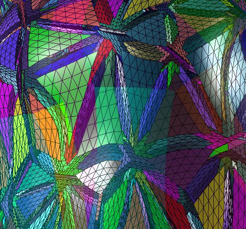
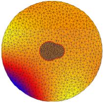
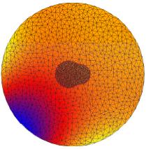
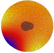
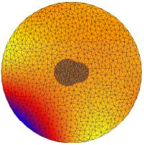
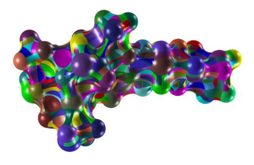
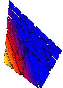
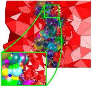
In the above figures, we show some results on a nonadaptive unstructured mesh
composed only of two atoms for illustration purpose. The first
figure show the exact solution. The following one is the result of the linear
Poisson-Boltzmann equation which is very inaccurate. The remaining figures show some
intermediate nonlinear results and the ultimate nonlinear approximation.
As for the hierarchical case, the nonlinear solver follow the same line just as
in the multiblock case with the exception that you have the cascading
advantage and the multiple level results.
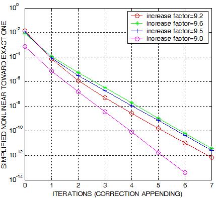
The right plots contain some outcomes for a model when enhanced with the
hierarchical strategy. The different curves are obtained for various number
of blocks on some levels. The
increase factor indicates the increase of the number of tetrahedra on the
inter-level hierarchical refinement. It is observed that on all tests that
we have done the converge is much faster than what it observed above in the
case of dispensing from hierarchical structure.
|
|
|
BFGS / FHT (BROYDEN-FLETCHER-GOLDFARB-SHANNO / FAST HARTLEY TRANSFORM):
|
The usual quasi-Newton use only an approximate Hessian. One of the widely
used approximate Hessian updates is the BFGS which are of two kinds:
direct one and the inverse one. They update respectively the
Hessian and the inverse of the Hessian at every iteration. The
direct BFGS still necessitates a solving of the approximate Hessian
at each iteration while the inverse one needs only one matrix-vector
multiplication. Still, the inverse BFGS is very much flawed by the
initialization because you need to have a pretty good approximation of
the initial inverse Hessian. In some problems, such an initial good
inverse is easy to obtain. In our case of Poisson-Boltzmann, it is very
expensive to assemble even the inverse of the initial Hessian.
Therefore, a direct BFGS is more reasonable in our case.
The drawbacks of using the direct BFGS update formula are:
- The resulting BFGS-matrices are not sparse. Hence, one would need
O(n2) memory space for the allocation.
- Although the matrix from the BFGS
updates is symmetric positive definite, its non-sparsity
makes it difficult to solve using fast solvers like CG or GMRES.
- Although the matrices are easy to update, the resulting matrices
are usually badly conditioned resulting to many iteration counts
- A single matrix-vector multiplication for a dense BFGS-matrix of
order n which represents the number of Finite Element unknowns
is very expensive.
|
|
One would like to keep the advantage of BFGS (easy update, no need to assemble full Hessian)
while trying to avoid the above drawbacks.
The main idea of the FFT-BFGS is to obtain an updating formula whose results are
easy to treat. First you need only
O(n) memory for the storage. On the
other hand, the matrix to be solved is diagonal after a few DFT or DHT transforms
which can be done very fast. The usual FFT based BFGS completely ignores the
initial matrices and makes an update. In our problem some part of the Hessian is
available and sparse. As a consequence, we apply only the FFT-BFGS update to the
non-sparse information.
|
Line search: the most usual ways of line searches are
Armijo, Goldstein, Powell, Cauchy,
etc. For our simplified nonlinear method, the line search equation is given as
a univariate polynomials of low degree. Searching the line search solution amounts
therefore to selecting between the few roots, which can be computed exactly, the
one minimizing the objective functional in the current search direction.
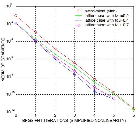
On the left plot, we see some convergence history of the resulting method.
Minimizing the functional necessarily amounts to detecting the position
of zero gradients. As a consequence, measuring the gradient norm an in the plot
is a good gauge of assessing the quality of the nonlinear solver.
We observe that the Quasi-Newton behaves very efficiently. The resulting FFT-QUASI-Newton almost
admits the convergence property of the exact Newton.
|
The above result admits the same property for both the unstructured and hierarchical
settings. Recall that the implementation of the DFT/DHT by the FFT method is already
hierarchical. The Cooley-Tuckey algorithm already implicitly 'halfen'
the data at every iteration.
|
ADAPTIVE REFINEMENT AND HIERARCHY:
|
We consider a-posteriori error estimates which can be computed very efficiently.
Although the initial problem is a nonlinear one, the a-posteriori error estimator
is a linear one. Based upon the strengthned Cauchy-Schwartz inequality, one
can deduce an a-posteriori error estimator which is both
efficient
and
reliable. In other words, one can derive the next property
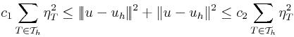
where the constants
c1 and
c2 are
independent of the discretization properties of the underlying mesh for two
local bases
V(T) and
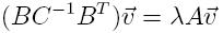
Z(T). The stiffness matrix with respect
to the bases of
V(T) and
Z(T) is given in
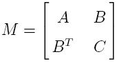
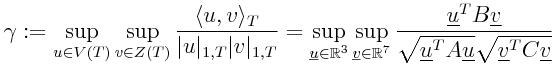
M as follows. In function of its block matrices, the original
strengthned Cauchy-Schwarz constant is expressed otherwise
Therefore, γ is given by the square root of the largest eigenvalue of
the generalized eigenproblem
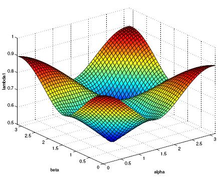
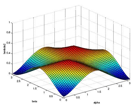
Here are some instance of the eigenfunctions of some well chosen
local decomposition:
- Parallel implementation: this extension is not difficult (but it takes time)
since everything in the sequencial version is already set blockwise. Hence, the
parallelization seems to be only a distribution of the blocks to the processors.
- Currently, the choice of polynomial degree is done by heuristic. More mathematical
way is needed to choose the degree as well as to decide between mesh refinement and polynomial
degree elevation.
- The a-posteriori error estimator always work in practice but the analysis
is only partially finished for the piecewise linear case.
- Improvement and optimization of the code.
- Papers.